

Impact of the Microphysics in HARMONIE-AROME on Fog
by
 , , , and
Sebastián Contreras Osorio
1,*,
Daniel Martín Pérez
2,
Karl-Ivar Ivarsson
3,
Kristian Pagh Nielsen
4,
Wim C. de Rooy
1,
Emily Gleeson
5 and
Ewa McAufield
5 1
Research & Development Weather and Climate Models, Royal Netherlands Meteorological Institute (KNMI), P.O. Box 201, 3730 AE De Bilt, The Netherlands
2
Agencia Estatal de Meteorología (AEMET), 28071 Madrid, Spain
3
Swedish Meteorological and Hydrological Institute (SMHI), SE-601 76 Norrköping, Sweden
4
Danish Meteorological Institute (DMI), DK-2100 Copenhagen, Denmark
5
Irish Meteorological Service (Met Éireann), 67 Glasnevin Hill, Glasnevin, D09 Y921 Dublin, Ireland
*
Author to whom correspondence should be addressed.
Atmosphere 2022, 13(12), 2127; https://doi.org/10.3390/atmos13122127
Submission received: 12 October 2022
/
Revised: 6 December 2022
/
Accepted: 12 December 2022
/
Published: 19 December 2022
(This article belongs to the Special Issue Decision Support System for Fog)
Abstract
:This study concerns the impact of microphysics on the HARMONIE-AROME NWP model. In particular, the representation of cloud droplets in the single-moment bulk microphysics scheme is examined in relation to fog forecasting. We focus on the shape parameters of the cloud droplet size distribution and recent changes to the representation of the cloud droplet number concentration (CDNC). Two configurations of CDNC are considered: a profile that varies with height and a constant one. These aspects are examined together since few studies have considered their combined impact during fog situations. We present a set of six experiments performed for two non-idealised three-dimensional case studies over the Iberian Peninsula and the North Sea. One case displays both low clouds and fog, and the other shows a persistent fog field above sea. The experiments highlight the importance of the considered parameters that affect droplet sedimentation, which plays a key role in modelled fog. We show that none of the considered configurations can simultaneously represent all aspects of both cases. Hence, continued efforts are needed to introduce relationships between the governing parameters and the relevant atmospheric conditions.
1. Introduction
Fog is an atmospheric phenomenon that can have a high impact on human activities, such as aviation or road and maritime transport [1,2,3], due to the reduction in visibility caused by small water droplets. The life cycle of fog is influenced by numerous processes, spanning multiple spatial and temporal scales [1,4,5,6,7,8]. Among the involved processes are the nucleation of aerosol particles, surface heat, and water fluxes, turbulence, radiative cooling, sedimentation by gravity, etc. The interplay between these processes restricts the correct simulation and forecast of fog. In particular, numerical weather prediction (NWP) models have difficulties in reproducing the timing of fog formation and dissipation, as well as spatial features including the spread of fog and its exact location [3,9,10,11,12]. Consequently, fog forecasting remains a major problem at operational weather centres [13].
Due to the existing limitations concerning fog forecasting using deterministic NWP models, to date, various alternatives have been explored including ensemble prediction systems (EPS) and observation-based techniques; see e.g., [14,15,16,17]. However, these methods have their own limitations (see, e.g., the previously cited references) and NWP models remain a crucial tool for end users. Consequently, a thorough analysis of the shortcomings of these models and their possible refinement remains a priority.
Deficiencies in the relevant parameterisations and the interactions between them are some of the main obstacles that limit the model’s performance regarding fog. A clear challenge is to find settings that work well for many cases [11]. In general, the improvement of parameterisations represents a major problem since atmospheric models are highly optimised and include several compensating errors [18,19,20].
The representation of low clouds and fog has been recognised as a persistent deficiency in the operational HARMONIE-AROME (HIRLAM-ALADIN Research on Mesoscale Operational NWP in Euromed–Applications of Research to Operations at Mesoscale) model [20,21]. This convection-permitting model was developed as part of a collaboration between the HIRLAM (High-Resolution Limited Area Model) and ALADIN (Aire Limitée Adaptation Dynamique Développement International) consortia. (Since 2021 this partnership has evolved into ACCORD (a consortium for convection-scale modeling research and development; http://www.umr-cnrm.fr/accord/) (accessed on 12 October 2022)). A detailed description of the HARMONIE-AROME cycle 40 is provided in [21]. This reference includes, in particular, a review of the physics parameterisations in the model.
An in-depth revision of the boundary layer schemes (cloud, turbulence, and shallow convection) has been recently introduced by [20], with the aim of improving the insufficient forecasting of low clouds. HARMONIE–AROME cycle 43 includes these modifications as the default configuration. The cloud microphysics scheme and fog were not considered in the aforementioned revision of the model and this motivates the present study.
The microphysical aspects of fog evolution remain poorly understood and this results in forecast limitations [8,17,22]. The atmospheric conditions governing different types of fog are highly variable, e.g., the type, number, and distribution of aerosols [23,24]. These variable conditions are not (or are only very roughly) considered in the aerosol representation in various atmospheric models with one-moment bulk microphysics schemes, such as in HARMONIE-AROME [25,26]. A central aspect of bulk microphysics schemes is the representation of hydrometeor size distributions by specified functions [27]. However, the shape of the cloud droplet size distribution, for example, is a rarely modified part of bulk parameterisations but can have a substantial impact on model output; see the recent studies of [13,28].
The purpose of this paper is to examine the role of the HARMONIE-AROME cloud droplet representation under fog situations. In particular, we focus on the microphysical aspects of cloud droplets in the model. We consider the impacts of two aspects of cloud microphysics: (1) recent modifications to the characterisation of the cloud droplet number concentration (CDNC), and (2) the parameters governing the shape of the cloud droplet size distribution. A particular objective of this work is to investigate the sensitivity of the model to microphysics parameters that can be implemented in ensemble forecasts in, e.g., stochastically perturbed parametrisation schemes. This represents the first step in the development and improvement of these schemes.
The present study is organised as follows. Section 2 introduces the microphysics aspects of cloud droplets in HARMONIE-AROME and the experiments to be performed. Subsequently, we describe two case studies of fog over the Iberian Peninsula and the North Sea in Section 3. Thereafter, the results of the experiments and a shared discussion regarding the two case studies are presented in Section 4 and Section 5, respectively. The latter section also outlines some future research possibilities that are motivated by the presented experiments. Finally, conclusions are drawn in Section 6.
2. Methods
The single-moment microphysics scheme in HARMONIE-AROME was originally developed at Météo-France and is based on [29,30]. The microphysics parametrisation is inherited from the Meso-NH model and can be summarised as a three-class ice parametrisation (ICE3) coupled to a modified Kessler scheme [31] for the warm processes. In particular, the transfer of cloud droplets to raindrops, autoconversion, is parameterised following [32]. The scheme considers five hydrometeors: cloud droplets, raindrops, cloud ice, snow, and a combination of graupel and hail. For a general overview of the microphysics scheme, see [33,34,35], and see [21,36,37,38] for specific modifications within HARMONIE-AROME.
The remainder of this section has the following structure: Section 2.1 introduces the two analysed configurations of cloud droplet number concentration (CDNC) and shape parameters of the cloud droplet size distribution. The link between these parameters and sedimentation is examined in Section 2.2. The six considered experiments in this study are introduced in Section 2.3.
2.1. Cloud Droplet Characterisation in HARMONIE-AROME
Three parameterisations in the microphysics scheme of HARMONIE-AROME take into account the CDNC. These are the parameterisations of autoconversion, collision, and sedimentation of cloud droplets. In this work, we focus on sedimentation, given its major role in fog development, as will be discussed in subsequent sections. The microphysics scheme in HARMONIE-AROME represents the cloud droplet size spectrum by the following generalised gamma distribution:
with D the diameter, the gamma function, N the total cloud droplet number concentration (also referred to as CDNC here), the slope parameter, and the distribution shape parameters. can be calculated from the predicted moment (i.e., the mass mixing ratio) and the other distribution parameters. The shape parameters define the shape of the size distribution, which means that these parameters control the relative amount of droplets of different sizes.
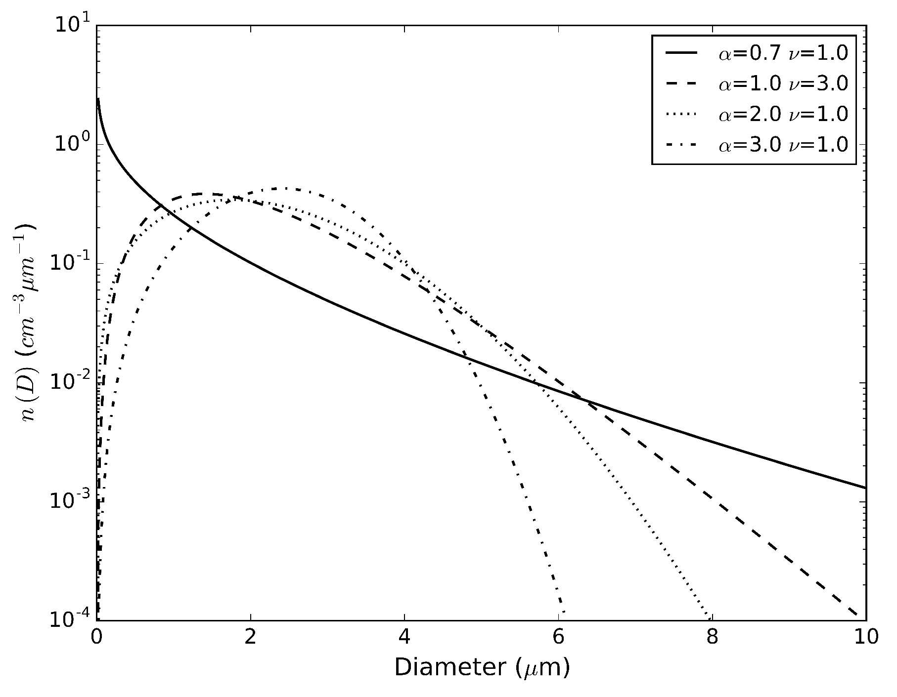
Figure 1 shows examples of the generalised gamma distribution for the and values that will be considered in the experiments introduced in Section 2.3. In particular, it can be seen from the figure that the number of large droplets increases for lower values of . This increase in the number of large droplets leads to an increase in sedimentation. Note that when , the size distribution (1) reduces to a gamma distribution; if in addition , the spectrum becomes an exponential distribution. The latter is adopted in the microphysics scheme for raindrops, snow, and the combination of graupel and hail; for cloud ice, . See [33,39] for further details. (The terminology in cloud microphysics regarding the generalised gamma distribution (and its parameters) is not fixed and different expressions and symbols are used in the literature. For a more general discussion on the generalised gamma distribution, see [40,41,42,43].)
In the microphysics scheme of HARMONIE-AROME, the values of the shape parameters for cloud droplets and CDNC have been given values based on the geographical region (sea, land, and urban) in order to, indirectly, take into account the different populations of cloud condensation nuclei, see e.g., [44,45]. A study presented in [44] considers the possible impact of the difference between maritime and continental settings near the coast for fog. The exploration in the cited study includes fixing the same values for parameters N, , and for both the sea and land regions; a clear conclusion made by the authors, is the impact of the different distributions of sedimentation, which- affects the modelled liquid water content and the location of fog.
Intuitively, the impact of varying the shape parameters or CDNC on the size distribution and sedimentation can be understood as follows. Lowering these parameters for a fixed liquid water content results in a greater number of larger droplets at the higher end of the size distribution, which implies faster sedimentation; the opposite is true when the values of the parameters are increased, see, e.g., [44,46].
The shape parameters were originally regarded as adjustment parameters that take on fixed values, see, e.g., [47]. This is a general characteristic of bulk microphysics schemes: some parameters of the size distribution need to be either fixed or determined using additional (semi-empirical) relationships due to the calculation of only a limited number of moments of the distribution [42]. In fact, the performance of bulk microphysics schemes highly depends on the realism of the assumed size distribution (and its associated parameters) [48]. The wide range of parameter values reported in the literature, e.g., [46,49,50,51,52] motivates the experiments that will be considered in this study. Previous explorations of different values of the shape parameters in the context of this investigation revealed that these parameters can impact the modelled fog. In particular, the characteristics that can be influenced are the horizontal extension, vertical growth, and visibility. Some representative experiments are selected in this study to illustrate the impact of the shape parameters on fog cases. We focus on the impact of above sea and, in particular, we will consider a case with a low given the reported values of () for fog in [49,51,53].
The assumed functional form of the size distribution of the different hydrometeors, combined with power laws for the mass- and velocity-size relationships, allows analytical calculations and computational efficiency. The configuration of CDNC values and size distribution parameters in the HARMONIE-AROME model has been recently modified in cycle 43h2.2 (although it is still possible to use the original configuration). Both configurations are described below.
2.1.1. Constant CDNC
In this configuration, constant values are set for different land cover types: 100 cm−3 over the sea, 300 cm−3 over land, and 500 cm−3 over urban areas. The size distribution parameters ( and ) are constant as well, with equal to 3 over the sea and 1 over land, with equal to 1 over the sea and 3 over land. Given the parameter values, the droplet size distribution is fixed in space and time in this configuration.
Moreover, in this configuration, an inconsistency with the CDNC used in the radiation scheme must be mentioned. In the radiation scheme values of 50 cm−3 over the sea and 313 cm−3 over land and urban areas are used. Since there is no vertical dependence of the CDNC in this configuration, an indirect decrease of aerosols with height is not considered. Neither is the dependence of the CDNC with supersaturation, which is responsible for the activation of the cloud condensation nuclei (eventually increasing the number of available nuclei to form cloud droplets).
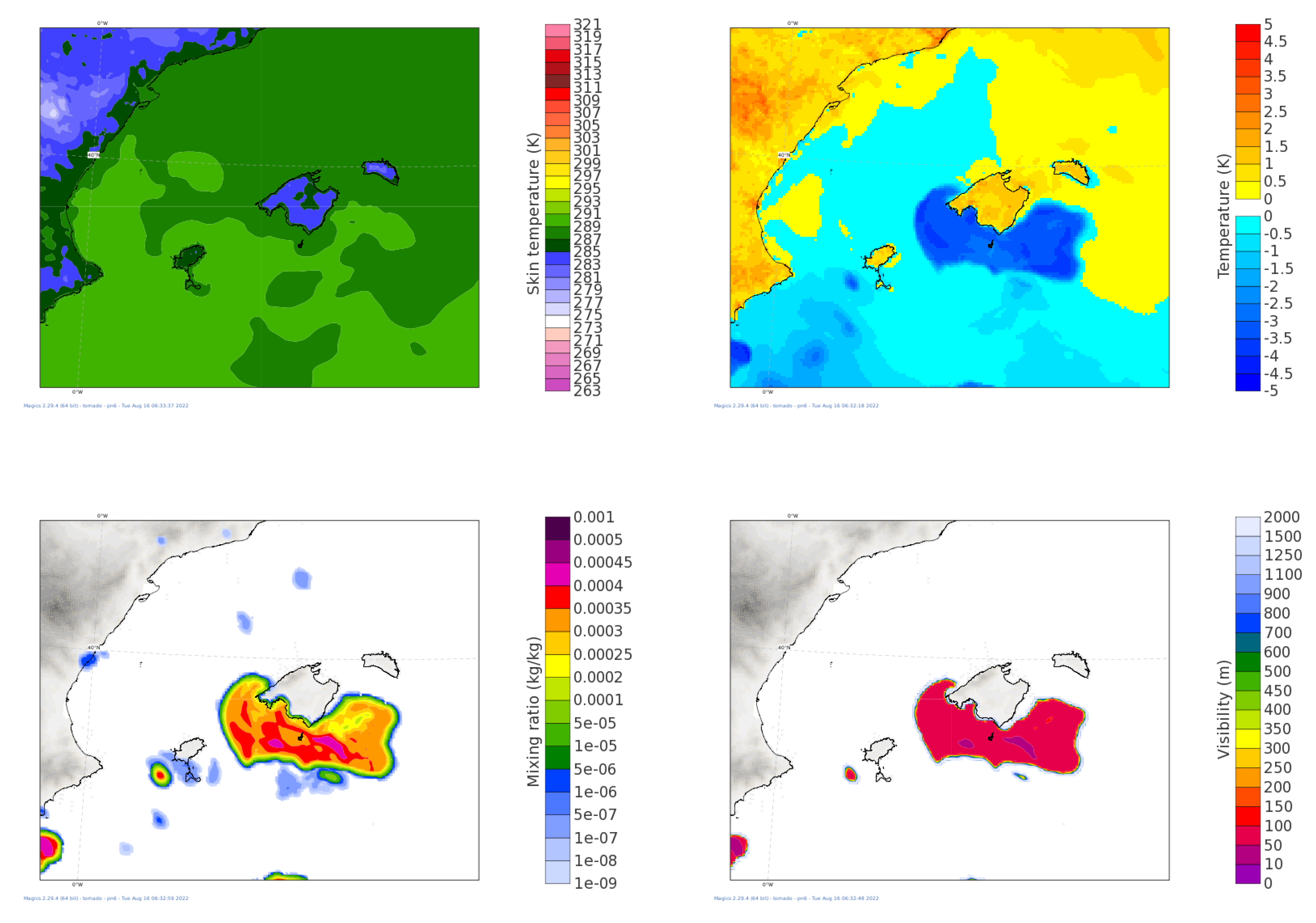
The values of CDNC seem to be, in general, too high for fog in this configuration (see e.g., [54]). Occasionally, the model develops incorrect or spurious fog over the sea. Such fog is characterised by a high cloud water content, low temperature, fast growth, and round-shaped contours. It forms at the coast or over land and starts to grow faster once it reaches the sea. Figure 2 (top row) shows an example of this situation in which the constant CDNC configuration was applied; this case will be further considered in Section 2.3 and referred to as ‘CONST_DEFAULT’ experiment.
Moreover, drizzle discontinuity problems at the coast (land–sea split), due to the change in the CDNC between sea and land, also motivate some modifications to this configuration. The second configuration considered in this study, ‘variable CDNC’, will be introduced in the following subsection.
Examples of the liquid–water mixing ratio and visibility are shown in Figure 2 (bottom row). HARMONIE-AROME assumes a relationship between visibility and the extinction coefficient given as a function of hydrometeor content. Empirical expressions between the extinction coefficients and the density of hydrometeors are used following [55,56]. Additionally, a combination of the relative humidity and an estimation of the cloud condensation nuclei (CCN) is used when hydrometeor concentrations are zero [57]. In order to exhibit the impact of the different experiments considered in this study, we will present the cloud fraction at the lowest model level, the low cloud fraction (Iberian Peninsula case), and the liquid–water mixing ratio (North Sea case). Low clouds are defined as those with a cloud base height lower than 2000 m in the WMO’s International Cloud Atlas [58]; this definition is followed in this work.
2.1.2. Variable CDNC
A new profile of CDNC was implemented in order to make the CDNC consistent in both the microphysics and radiation schemes, to avoid the previously mentioned discontinuity at the coast, and to have a more realistic vertical dependence:
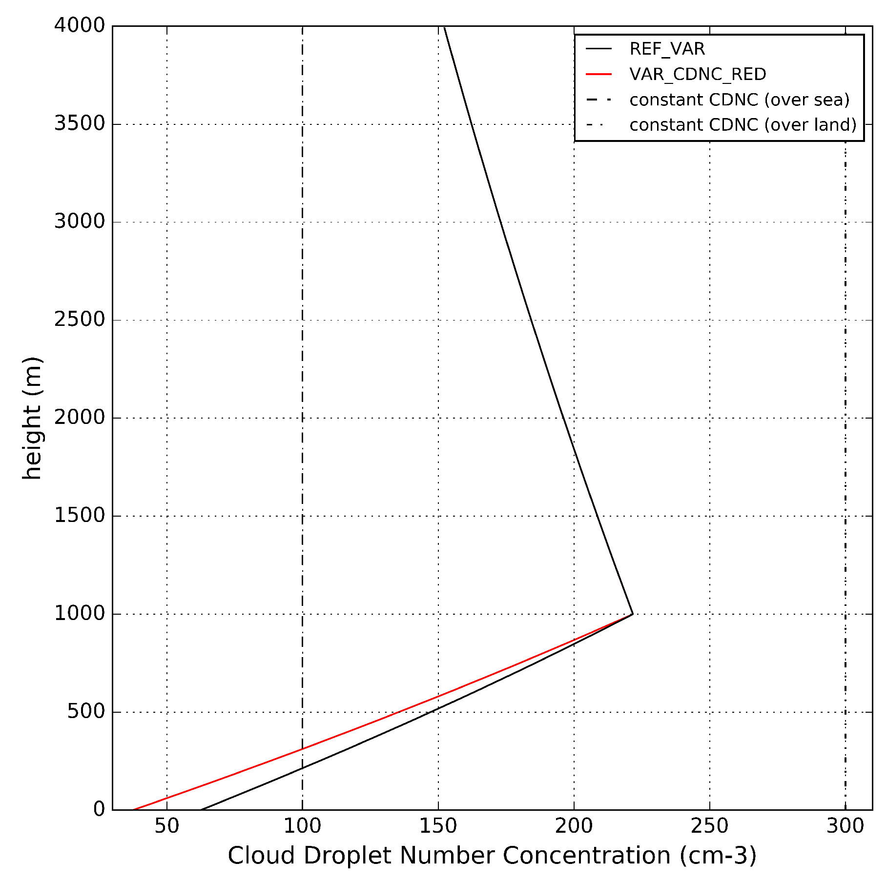
where P is the pressure, is the surface pressure, h is the height, H is the taper height (indicating the region, from the height above the ground, where an increase in CDNC will occur; considered to be by default), is the reduction applied to the CDNC at the surface and is the general value of cloud droplet number concentration. This general value is obtained at when no reduction () is applied. This configuration uses the same CDNC profile over the sea and land. Regarding vertical dependence, the CDNC is reduced proportionally to the pressure, for model levels below the taper height. That is, the CDNC is reduced while approaching the surface following Equation (2); see Figure 3. Two examples of the variable CDNC profile with different are displayed in this figure. The shown examples are referred to as ‘REF_VAR’ and ‘VAR_CDNC_RED’ in Section 2.3.
Cloud droplets form on activated aerosol particles so that the activated nuclei mainly determine the number of cloud droplets. However, the number of activated nuclei depends not only on the total number of aerosol particles that can behave as condensation nuclei (e.g., sea salt, sulphate, etc.), but also on the supersaturation conditions that activate those nuclei. The diminution of the CDNC with pressure in Equation (2) pretends to take into account the fact that aerosol sources are located at the surface. The maximum of CDNC is consistent with the fact that the supersaturation values at the surface are not as high as they can be inside the clouds, see e.g., [59]. As the supersaturation increases with the vertical velocity, more aerosols can be activated due to adiabatic cooling (simulations of the droplet spectrum evolution in (cumulus) clouds can be found in [60]). See also the discussion in [9] where a tapered curve is introduced to represent the vertical CDNC profile. In the absence of updrafts, a profile representing the diminution of CDNC with height with no absolute maximum would be more likely to be found. This kind of profile can be obtained for values of closer to 1.0, although this is not considered in this study. Moreover, drizzle also drains out the condensation nuclei, reducing the possibility of the formation of new cloud droplets.
Concerning the size distribution parameters, although the parameter values for sea and land are kept inside the code (by default: , over the sea; , over land), different values are used in practice. These effective values result from the calculation of a linear mean of functions that are necessary for the calculation of sedimentation (a similar mean is considered in the constant CDNC configuration where a combination of land and sea fractions is present). In the new configuration, the effective values are obtained by considering equal land and sea fractions of 1/2. Exploratory tests for fog cases that take into account different combinations of parameter values showed that using and for both sea and land results in a similar behaviour to that when the previously mentioned default values (different over the sea and land) are used. We refer to and as the ‘effective values’ for the variable CDNC configuration.
2.2. Parametrisation of Sedimentation
It has been shown that sedimentation is a key process in the development of fog and models that include droplet settling generally result in better model performances; see, for example, [9,13,34,61,62]. The sedimentation scheme in HARMONIE-AROME is introduced in [62]. The algorithm was developed at Météo-France and considers transfer probabilities that take into account the hydrometeor content at different model levels.
The parametrisation of sedimentation uses CDNC and the shape parameters of the cloud droplet size distribution (Equation (1)). In particular, the sedimentation depends on the terminal velocity of the cloud droplets. In the Stokes regime, the terminal velocity of a droplet is proportional to the square of the radius [63]. The mean value of the terminal velocity for the distribution of droplets can be obtained as follows:
where r is the droplet radius, C is a parameter depending on gravity, the densities of water and air, and the dynamic viscosity, is the liquid water content, is the water density, and N is the CDNC. In the HARMONIE-AROME model, a correction term for very small droplets is also considered but it is not critical for the general behaviour.
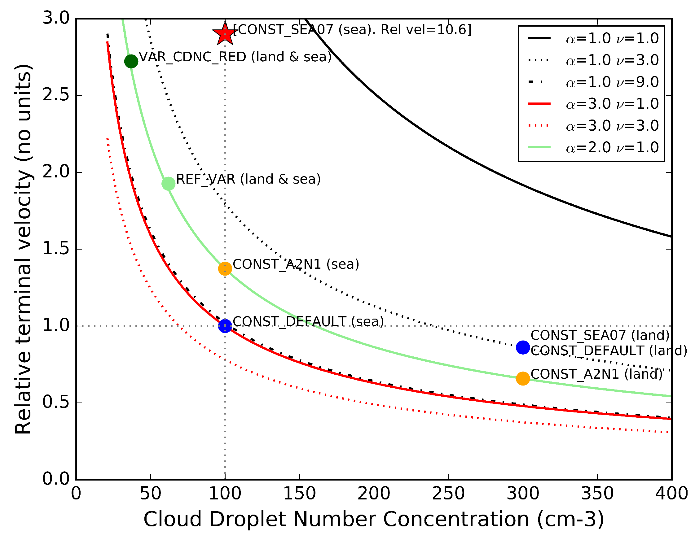
Figure 4 shows the relative terminal velocities as a function of the CDNC for different values of the parameters of the size distribution. An increase in the terminal velocity increases the sedimentation. As expected, a reduction in the CDNC increases sedimentation, while, for the same values of , increasing the value of reduces the sedimentation.
2.3. Description of Experiments
In order to compare the two CDNC configurations and to illustrate the impacts of the shape parameters of the size distribution, we consider six experiments that are summarised in Table 1. The same experiments are performed for the two cases described in the following section in the domains of the Iberian Peninsula and the Netherlands. In the sensitivity experiments, a horizontal grid spacing of 2.5 km and 65 vertical levels are considered with the lowest level at approximately 12 m. (Although the lowest level height is higher than that used by other models (see e.g., [13]), this is currently used for fog characterisation at AEMET and KNMI. Research on the impact of modifying the height of the lowest level is worthwhile but beyond the scope of this study.)
The REF_VAR experiment represents the default configuration of the HARMONIE-AROME model. This experiment adopts the variable CDNC profile and the same shape parameter values for sea and land (see Section 2.1.2). Since CONST_DEFAULT adopts the constant CDNC configuration (with different shape parameters for sea and land), these experiments enable the comparison between the two main microphysical settings.
CONST_A2N1 is considered in order to exemplify the impact of having a constant CDNC with the same values of the shape parameters (i.e., , ) for both sea and land. Moreover, these values roughly correspond to the effective values of the shape parameters in REF_VAR. The comparison between CONST_A2N1 and REF_VAR allows us to study the impact of changing the constant configuration of CDNC to the one that varies with height.
Above sea CONST_DEFAULT, CONST_A2N1, and CONST_SEA07 represent reductions in the shape parameter . The value of in CONST_SEA07 is selected as an example of and is motivated by such values reported in the literature (see Section 2.1). Experiment VAR_CDNC_RED is selected as an example of further reducing the value of the CDNC at the lowest model level by reducing the parameter. This modification implies a reduction in the CDNC at the surface from 62.5 cm−3 for REF_VAR (and VAR_NOSED) to 37.5 cm−3 for VAR_CDNC_RED (see Figure 3). Finally, VAR_NOSED is included in order to additionally display the impact of the sedimentation of cloud droplets on modelled fog. In this experiment, the sedimentation of cloud droplets is deactivated.
The results of the experiments will be compared with the satellite images that introduce the case studies in the following section. The nature of this comparison is qualitative and seeks to highlight general characteristics and motivate a discussion on the main differences between the experiments.
3. Case Studies
In this study, we consider two fog situations in order to analyse the impact of the microphysical representation of cloud droplets in HARMONIE-AROME. In the first case, in the Iberian Peninsula, we consider an example with fog and low clouds over both sea and land. A situation in the North Sea is considered as second case showing an example in which the spatial extent of the fog predicted by the model is much larger than observed.
3.1. Iberian Domain
The Iberian domain extends approximately from 30° to 50° north and from 20° west to 10° east. It covers the whole Iberian Peninsula, the south of France, and the west of the Mediterranean Sea, as interest zones for our study. The Iberian Peninsula has a complex orography. There are two plateaus in the centre of the Peninsula with mean altitudes of 750 m for the north plateau, and 600 m in the case of the southern one. These, together with the Ebro valley in the northeast, are the main areas of fog development in this case. The Atlantic coast of the south of France is another zone of interest. It is relatively flat and the influence of the ocean is important.
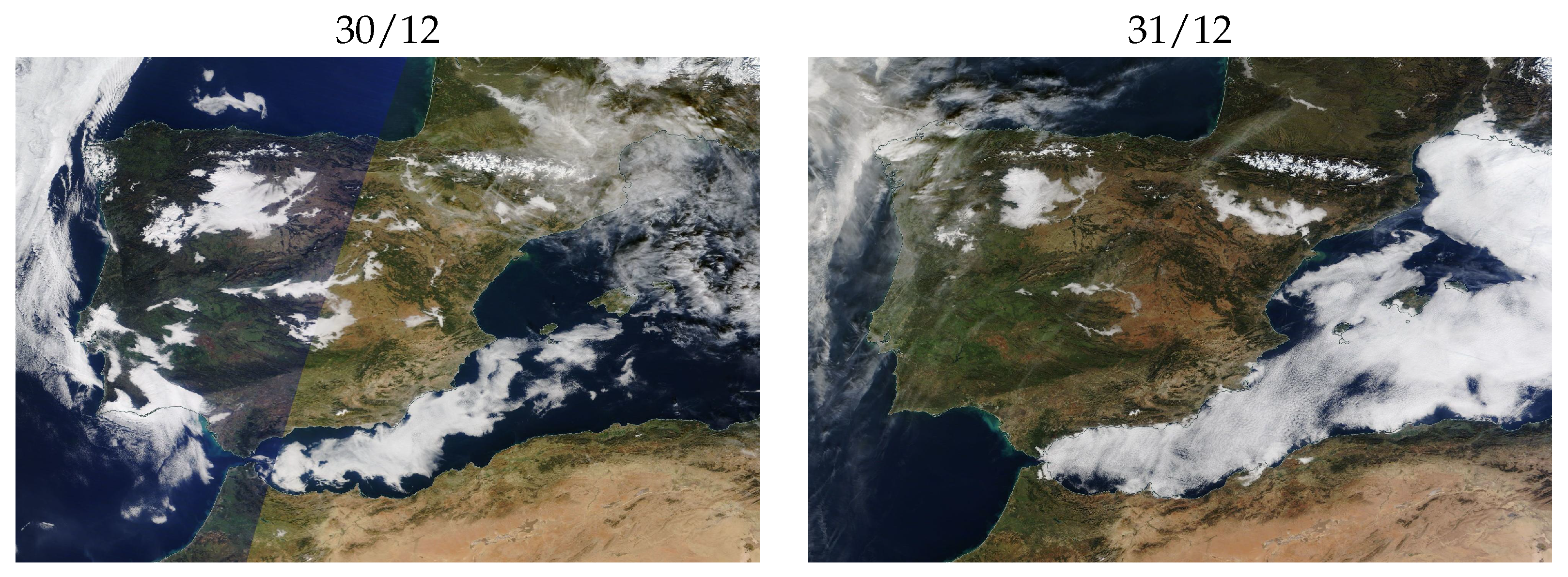
December 2021 was a month characterised by very stable weather and fog development over the Iberian Peninsula. At the end of the month, from the 29 to 31 December, a high-pressure system was dominant, keeping any fronts approaching from the west far away from the coast. At noon on the 29th, fog and low clouds covered the north and south plateaus but were already in the dissipation stage. The spatial extent reduced until only the southwest of the peninsula and a few areas in the Alboran Sea (at the southwest of the Mediterranean Sea) were covered at midnight. Fog and low clouds started to develop again during the early morning of the 30th. At 11 UTC on the 30th (Figure 5, left) the fog was present again over land over both plateaus and the southwest of the peninsula.
As was the case the previous day, the clouds started to dissipate, and only an area of the northern plateau was cloudy until night, while the extent of the low clouds and fog over the Mediterranean Sea kept increasing until a large part of the sea between the Balearic Islands and the Iberian coast was covered. On the 31st, the fog and low clouds covered a large area of the Mediterranean Sea again while the spatial extent of the fog over land was not as large as the previous day (Figure 5, right).
3.2. North Sea
The Netherlands domain is centred at the Cabauw experimental site for atmospheric research (51.97° N, 4.9° E) in the western part of the country. It covers a large part of western Europe and the North Sea. This latter region is particularly important in terms of fog in the Netherlands due to maritime transport, offshore wind infrastructure, and the location of the main airport close to the coast. More generally, the North Sea greatly influences weather conditions in the Netherlands due to the uniform topography and absence of significant terrain barriers.
The 2012 fog case introduced in [64,65] is considered a representative situation of a persistent fog field above sea that was over-predicted by the model, particularly in its spatial extent. Previous experiments considering this fog situation explored different processes that could be related to the formation of excessive fog in the model (e.g., the convection and turbulence schemes) [64]. We consider this fog example again to study the impact of the two different CDNC configurations and the parameters of the size distribution mainly above sea.
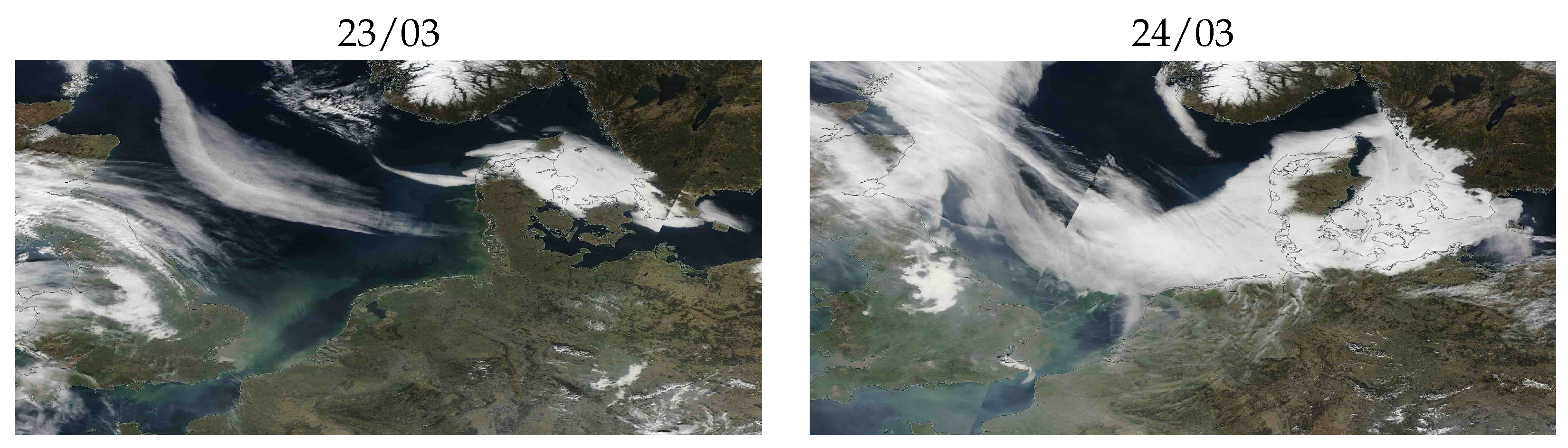
The synoptic situation was characterised by a high-pressure region to the north of the Netherlands over the North Sea. From satellite imagery, no fog was present at the start of the experiments. One day after, at approximately 11 UTC on 23 March, a small region of fog near the coast of Denmark expands towards the North Sea. Moreover, a band of low clouds and possibly some fog can be observed between the northwest region of the North Sea and the west coast of Denmark, see the central region of Figure 6 (left). On 24 March at approximately 11 UTC, a larger region of fog can be observed to the north of the Netherlands that stems from the fog field that was present close to Denmark the day before, see Figure 6 (right).
4. Results
4.1. Iberian Domain
A 48 h period from 29 December at 12 UTC was selected. The experiments presented in this subsection were run with a warm start, i.e., the initial conditions were taken from the operational HARMONIE-AROME model run at AEMET. This ensures that the experiments do not start with spurious instabilities. (The operational model is based on cycle 43h2.1.1 whose microphysics parameters are those corresponding to the CONST_DEFAULT experiment, see Table 1). The operational model produced more extensive fog over land but dissipated the fog earlier compared with the observations. Moreover, in the operational model, incorrect or spurious fogs that grow in spatial extent at longer forecast times were developed over the sea around the Balearic Islands and the north African coast (similar to the situation displayed in Figure 2).
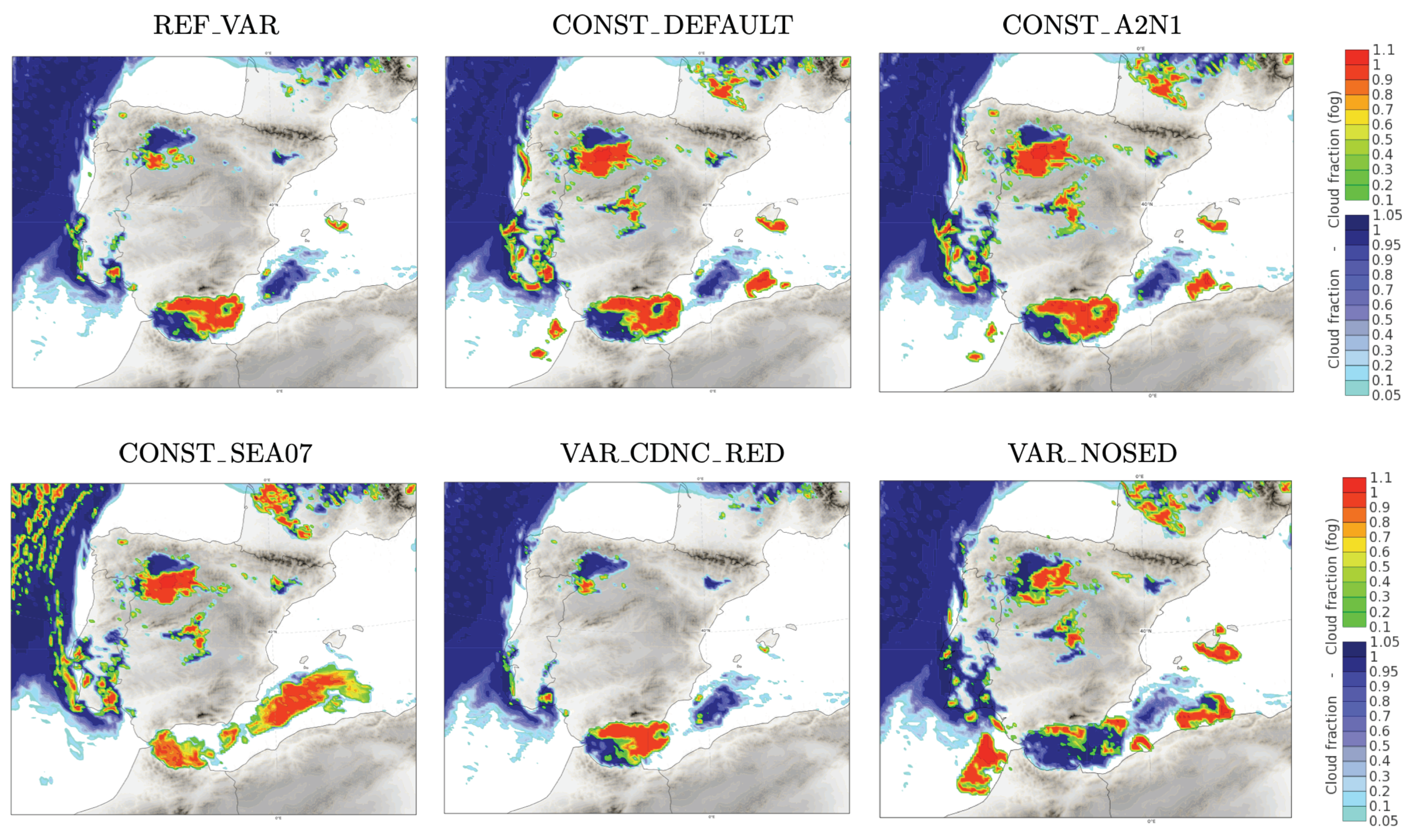
Figure 7 shows the fog (cloud fraction at the lowest model level) and low clouds for the different experiments after 23 h of integration over the Iberian domain. When comparing the forecasts from the different experiments (Figure 7) with the satellite image at 11 UTC on 30th December (Figure 5, left), differences over land are noticeable. REF_VAR and VAR_CDNC_RED have lower spatial extents of the fog and low clouds over land due to the lower CDNC near the surface. This decrease in CDNC when using the variable CDNC profile increases the sedimentation in the lower levels of the model (the cloud droplet terminal velocity is higher in these experiments than in CONST_DEFAULT; Figure 4) and reduces the cloudiness. CONST_DEFAULT, CONST_A2N1, and CONST_SEA07 have similar distributions of fog and low clouds over land and are more similar to the observations. VAR_NOSED, where the sedimentation was deactivated, shows a similar distribution of clouds over land to the previous experiments but with more low clouds than fog.
Over the sea, CONST_SEA07, where the sedimentation increases by increasing the terminal velocity of the droplets via reducing the parameter, shows different behaviour from the other experiments. The cloudy area over the Alboran Sea has a similar areal extent to the rest of the experiments but it mainly consists of fog in this experiment. This is due to the increased sedimentation causing the cloud droplets to fall to lower levels where they can evaporate and increase the humidity. Consequently, water vapour may condensate, lowering the cloud base height or developing fog at a lower model level. A reduction in the cloud base height is also noticeable in the clouds to the west of the peninsula where, and only for this experiment, some patches of fog appear. Interestingly, for CONST_SEA07, spurious fog does not develop in the gulf of Cadiz in front of the Moroccan coast and to the south of Mallorca as occurs in the CONST_DEFAULT, CONST_A2N1 experiments and, especially, in VAR_NOSED.
After 47 h of model integration (Figure 8), similar conclusions are achieved. A reduction in the fog area over land for REF_VAR and VAR_CDNC_RED compared with the rest of the experiments is found. However, in the rest of the experiments, the spatial extent of fog is still lower than observed (see Figure 5, right). There is a complete lack of fog in the Ebro valley (the northeastern part of the Iberian Peninsula) for REF_VAR and VAR_CDNC_RED. Even VAR_NOSED with the sedimentation scheme deactivated is unable to reproduce the clouds over land (indicating that the model is not correctly developing fog in these areas). Furthermore, the fog that appears after the 47 h integration in southern France in CONST_DEFAULT, CONST_A2N1, CONST_SEA07, and VAR_NOSED, does not form in REF_VAR and VAR_CDNC_RED. This is probably because there is a lower CDNC in that area due to the advection of maritime air that REF_VAR and VAR_CDNC_RED can reproduce better. In the Gulf of Cadiz, CONST_DEFAULT, CONST_A2N1, and VAR_NOSED have developed spurious fog that does not form in the other three experiments, REF_VAR, CONST_SEA07, and VAR_CDNC_RED; see the left bottom region in the panels of Figure 8.
REF_VAR and VAR_CDNC_RED seem to exhibit better behaviour over the sea as spurious fog was reduced. (Note that in some regions, the CONST_SEA07 experiment also presents this behaviour.) However, they are not able to model the spatial extent of fog at increasing forecast times (e.g., at +047 h). Specifically over land, the reduction of the fog is excessive for these two cases, except in the south of France, which is more open to the influence of the sea (with generally ‘cleaner’ air).
4.2. North Sea
The experiments for the Netherlands domain were performed with a cold start on 22 March at 12 UTC and comprised a period of 48 h. In order to examine the impact of the different experiments on the 2012 case over the Netherlands domain, we present the liquid–water mixing ratio at the lowest model level for two different times +023 and +047 h. We focus on the North Sea since this area displays the main phenomena.
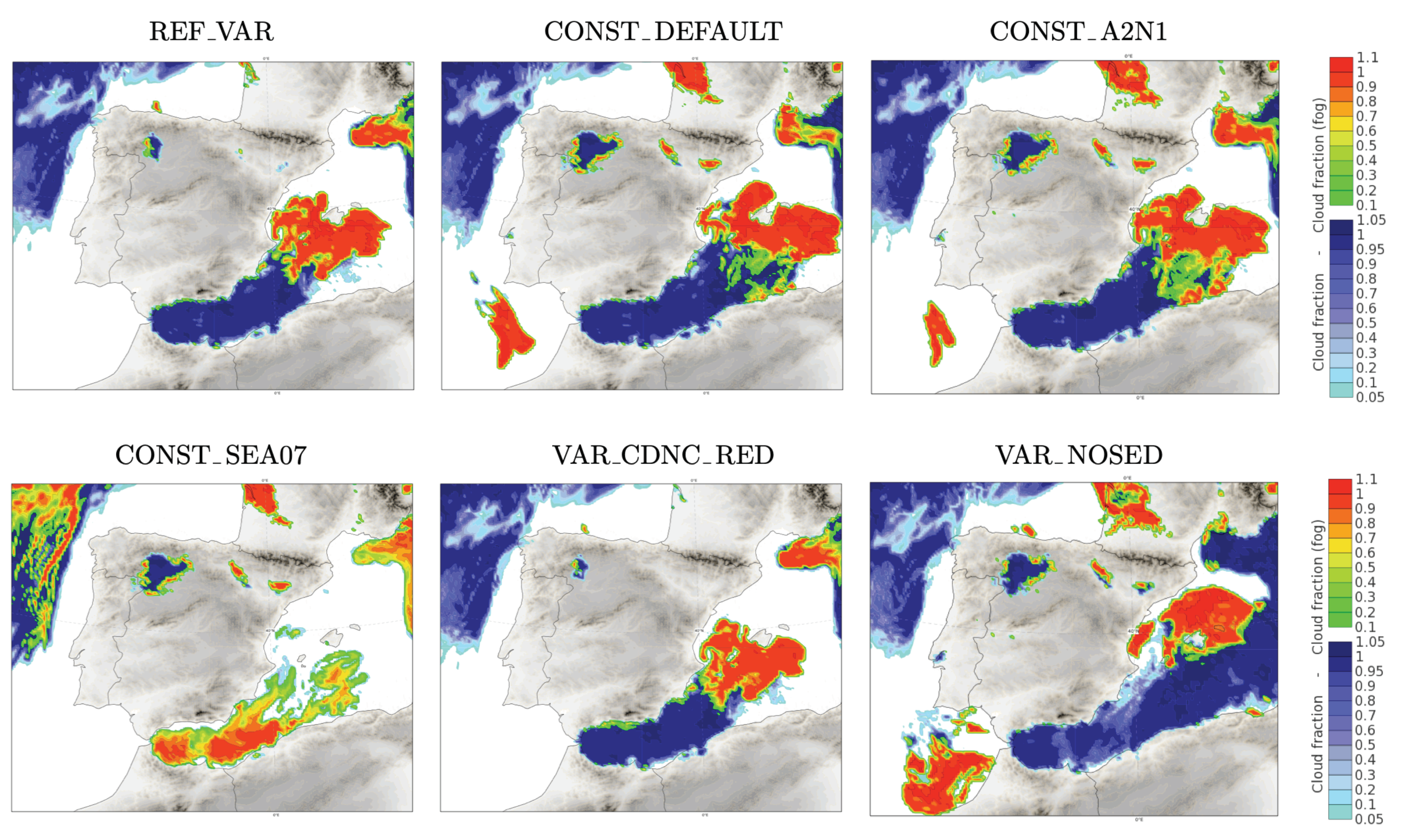
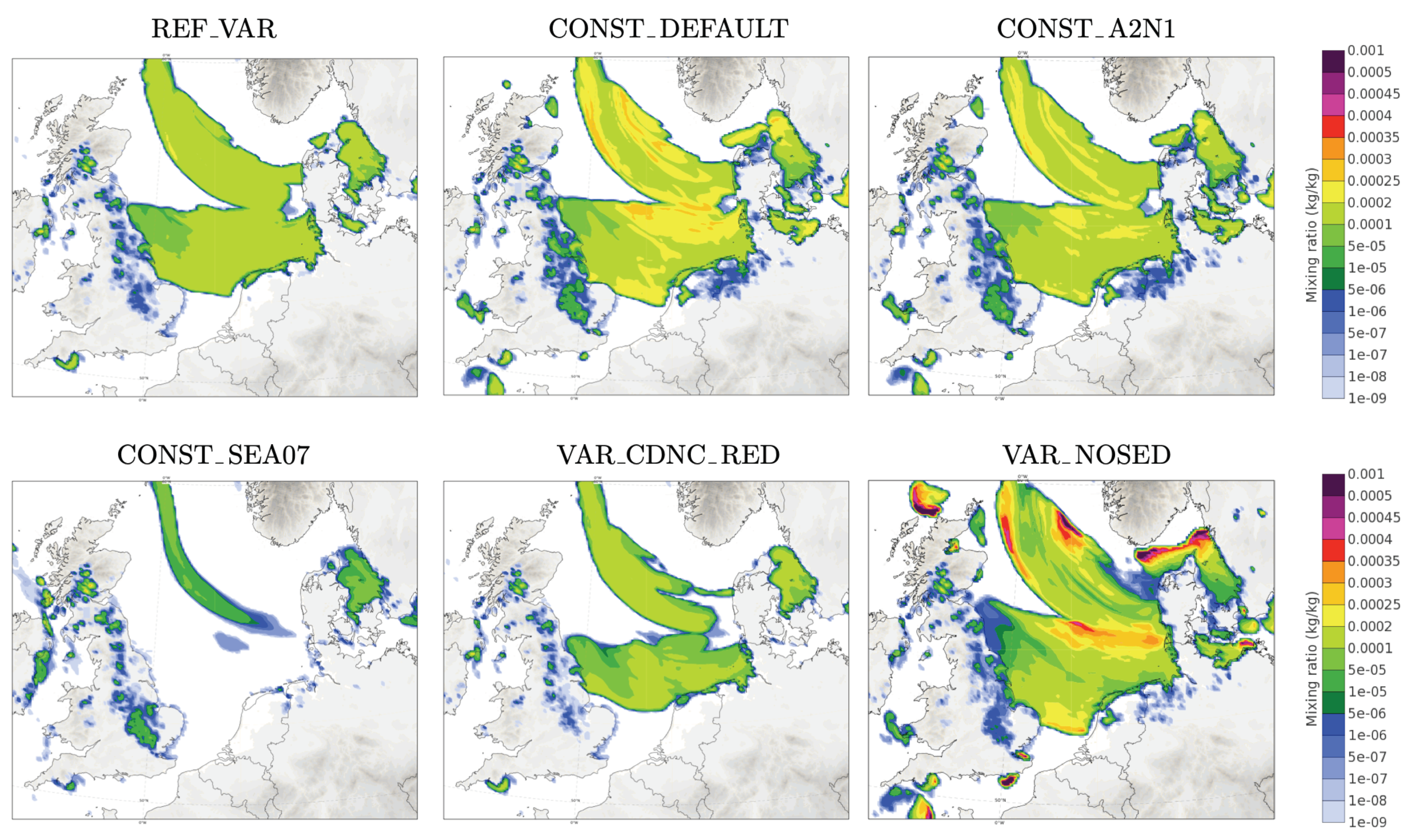
The general behaviour discussed in the case of the Iberian Peninsula is retained in the plots of Figure 9. Due to the modified CDNC, the REF_VAR experiment shows a reduction in water content compared with CONST_DEFAULT. CONST_A2N1 is similar to the previous cases in terms of the areal extent of fog but reduces the mixing ratio due to a slightly reduced above sea. An important difference between most of the experiments in Figure 9 and the satellite image (Figure 6, left) is the large extent of the modelled fog field. CONST_SEA07 is clearly an exception; a further reduced shape parameter for this case is able to highly limit the excessive expansion of fog.
Here, a clear feature of the impact when reducing can be noticed. While in the case of the Iberian Peninsula, a decrease in this parameter results in more fog above sea (where the low clouds turn into fog). In the North Sea case, the impact is the opposite, i.e., a reduction in the fog area. This is due to the presence of only fog in the latter case. That is, since influences all cloudy regions, the impact of this parameter on fog depends on the presence and location of other clouds.
Reducing the CDNC at the lowest level in VAR_CDNC_RED translates into a slight reduction in liquid water compared with the reference experiment REF_VAR. The situation displayed by VAR_NOSED clearly deviates from the rest, increasing the foggy region and showing the highest liquid–water mixing ratio. These characteristics, in disagreement with the satellite image, show the important sensitivity of the model to the activation of the sedimentation process.
Figure 10 shows the fog evolution after 47 h of model integration. In general, most of the experiments can be grouped as before where CONST_A2N1 represents an intermediate situation between REF_VAR and CONST_DEFAULT. VAR_CDNC_RED limits the expansion of fog shown by the REF_VAR experiment in the central part of Figure 10 and near Denmark. REF_VAR, CONST_DEFAULT, and CONST_A2N1 display a larger fog area in the west and southwest compared with the satellite image (Figure 6, right), and do not capture the region off the west coast of Denmark.
CONST_SEA07 and VAR_NOSED, where sedimentation is affected via the parameter and deactivated, respectively, show different characteristics from the rest. CONST_SEA07 shows hardly any fog (or low clouds) in the North Sea and VAR_NOSED shows an excessive area of fog in the English Channel region that is not observed. Moreover, VAR_NOSED does not reproduce the area with fog in the northwestern part of the North Sea (see Figure 6, right). In fact, a clear difference with respect to the rest of the experiments is that VAR_NOSED presents mainly low clouds throughout most of the North Sea (not shown). That is, the deactivation of sedimentation in this case increases the cloud base height and this translates into a reduction in the fog area. While the experiments CONST_SEA07 and VAR_NOSED present the smallest area of fog in the central part of the North Sea, the reason behind this is different for both cases. Namely, faster sedimentation in the former experiment, and an increase in the cloud base in the latter case.
Figure 9 and Figure 10 illustrate how some experiments represent fog better at certain forecast times and worse at others. The different models used operationally during this case showed similar behaviour. This exhibits the difficulty of finding specific CDNC and size distribution settings that work well in all cases. Therefore, this situation suggests the need to explore variable CDNC and size distributions since considering fixed values represents an overly restrictive assumption.
In general, the different experiments show similar behaviour in terms of fog to that of the Iberian Peninsula above land. (Note that in CONST_SEA07, there is no change in over land; the reduction of this parameter over land can also affect sedimentation (and fog), and this has been considered for other cases in the context of this research.) This has been observed for intermediate forecast times (e.g., +015 h) where fog regions form over land north of the Netherlands and Denmark (not shown). However, an important difference in the location of the fog region can be mentioned for VAR_NOSED and increasing forecast times (+033 h onward). This experiment shows a different distribution of fog and exhibits the highest amount of cloud water, which further manifests the different fog evolution in this case.
5. Discussion
This section has a two-fold purpose. Firstly, we present a discussion on the impact of the microphysics aspects on fog evolution as shown by the experiments. Secondly, possible future research directions are elaborated in light of the results.
The presented experiments were chosen in order to explore a high range of cloud droplet terminal velocities (as shown in Figure 4). The comparison between the three experiments with a constant CDNC profile allows us to analyse the impact of varying the shape parameters. From the experiments with a variable CDNC profile, two of them consider the impact of reducing the value of CDNC at the surface, and the third allows us to independently show the impact of sedimentation by deactivating it. The following list synthesises key aspects of the performance of the six experiments for both case studies.
- REF_VAR. In general, this experiment is able to partially reduce the areal extent of spurious fog over the sea. For the Iberian Peninsula, the spatial extent of fog over land is excessively reduced. Even though, this experiment is in agreement with observations in the south of France. For the North Sea, the fog extent is larger than observed but reduced in comparison with the experiments using the constant CDNC configuration.
- CONST_DEFAULT. This experiment reproduces in a better way the spatial extent of fog over the Iberian Peninsula. However, it predicts fog in the south of France that is not observed. Moreover, it develops unobserved fog in the Atlantic Ocean off the coast of Africa. In the North Sea case, the spatial extent of fog is larger than in the rest of the experiments; the cloud water content is also excessive in this experiment.
- CONST_A2N1. This experiment behaves in a similar way to CONST_DEFAULT over land and sea. It displays a lower spatial extent of fog and reduced cloud water content over the sea and, in general, the opposite behaviour over land. This can be understood by the modifications to the shape parameters that slightly increase sedimentation over the sea (and the opposite over land).
- CONST_SEA07. In general, this experiment behaves differently from the rest. As a negative point, the Iberian domain shows mostly fog in the Mediterranean Sea and underestimates low clouds. However, it removes the spurious fog off the coast of Africa. For the North Sea, the reduction of fog after 23 h is in good agreement with observations. However, it does not reproduce the observed fog at later forecast times (after 47 h).
- VAR_CDNC_RED. For the Iberian domain, this experiment shows a general reduction of fog which is positive in the south of France and off the African coast but not over the Iberian Peninsula. For the North Sea, this experiment reproduces the fog better, compared with REF_VAR, after 23 h and can be considered the second best (after CONST_SEA07). This experiment shows the best spatial distribution of fog after 47 h.
- VAR_NOSED. For the Iberian domain, in the Mediterranean Sea, the larger spatial extent of clouds reproduces the observation better. However, the spurious fog off the coast of Africa is more extended. For the North Sea, this experiment clearly deviates from the observations (and from the rest of the experiments), showing a different distribution of fog and the highest cloud water content.
A significant outcome that emerges from this synthesis is that the considered experiments cannot represent all aspects of the two fog cases. The use of the same CDNC over the sea and land for all domains seems to be too drastic. This deteriorates, in particular, the performance in certain regions over land far from the coast. Moreover, dense fog situations above land are likely to be underestimated due to the reduced CDNC close to the surface and the modified parameter value in REF_VAR. This generally results in reduced horizontal and vertical fog expansion and increased visibility. Running HARMONIE-AROME with the REF_VAR settings for several months at KNMI confirmed this underestimation of fog above land.
For the Iberian domain, the reduction in the spatial extent of fog over land is not desirable, therefore, high values of CDNC (over 200 ) are required. Most probably, the settings near the surface will not be implemented at AEMET. The results presented here, together with additional investigations taking into account different domains, point to the need to adjust the settings in REF_VAR and this is currently under investigation.
In the microphysics of HARMONIE-AROME, the shape parameters are only included in the sedimentation parametrisation. Additionally, the CDNC directly affects sedimentation, autoconversion, and collection of cloud droplets. A brief discussion of the other two microphysics processes is relevant. The collection of cloud droplets is responsible for the increase in rain intensity and, therefore, it is unlikely that this process has an important role in the considered cases with little precipitation.
Autoconversion is responsible for the initiation of drizzle [9]. The impact of the autoconversion can be analysed by comparing REF_VAR and VAR_NOSED, which use the same variable CDNC profile. Autoconversion depends on the CDNC and cloud water content [32]. Hence, the difference in the fog evolution exhibited by the two mentioned experiments is mainly caused by sedimentation and only in a secondary way, through the modification of the cloud water content, on autoconversion. This dependence seems to be indeed secondary for the Iberian case since the cloudiness increases for VAR_NOSED along all the integration. In the case of the North Sea, for VAR_NOSED the cloud water content has high values after 23 h at the lowest model level and this reduces significantly after 47 h. However, as mentioned in Section 4, the cloud base height and low clouds increase in the VAR_NOSED experiment. Differences in precipitation between the two experiments (not shown) are not critical, so we conclude that autoconversion has a secondary impact on this case as well.
In order to avoid an artificial distinction between continental and maritime air based on a land–sea mask, other options could be taken into account. The Tegen climatology [66], used by the HARMONIE-AROME model in the radiation scheme, makes a distinction between aerosol optical depth for maritime and land air and could be considered in order to have different CDNC vertical profiles and size distribution parameters for sea and land [67]. However, the Tegen climatology seems to have a too low resolution, and internal seas, e.g., are not well represented. For a good characterisation of the CDNC, detailed knowledge of the cloud condensation nuclei concentration in near real-time is required. The assimilation of aerosols from the Copernicus Atmospheric Monitoring Services (CAMS) [68] is currently in research mode in HARMONIE-AROME. This represents an interesting option to distinguish maritime and continental air; however, the computational cost is very high for operational purposes.
As shown in this study, the modification to the parameters of the size distribution can have a big impact on fog. Interestingly, the same modifications can lead to more (but also to less) fog, depending on the specific conditions. This reflects the indirect impact on the cloud base height. Comprehensive observations that specifically focus on the microphysical aspects (such as the real-time evolution of the droplet size distribution) could further guide model development. See [8,13] for a recent discussion on the need for more detailed measurements. Moreover, further studies need to be carried out in order to fully explore the impact of these parameters on other atmospheric situations. This exploration should also take into account the consistency between different schemes (e.g., microphysics and radiation).
An alternative to considering fixed values of the parameters of the size distribution is to implement additional dependencies between these parameters, examples of these relationships can be found in [2,69,70]. These relationships become increasingly interesting when more advanced microphysical schemes (higher moment bulk schemes) are considered. Further research using HARMONIE-AROME in this direction could be undertaken with the quasi-two-moment liquid ice multiple aerosols (LIMA) scheme [25,71] that will be available in future versions. (This scheme predicts, in particular, the number concentration of cloud droplets in addition to the mass mixing ratio.) However, the empirical relationships between the parameters of the size distribution are likely to have a limited validity range depending on the representativeness of the observations that motivate such relationships; see the discussion in [52].
An interesting approach to deal with the large uncertainty and impact of the shape parameters is to use them in ensemble prediction systems. These parameters have been introduced at KNMI in a stochastically perturbed parametrisation (SPP) scheme. SPP allows for the consideration of model errors that arise from the inaccurate representation of physical processes and parameter uncertainties. Preliminary results indicate a significant impact of the parameters, especially during winter, where they mainly affect cloud and fog-related variables. The performances of the SPP scheme (for different geographic domains) including the shape parameters are currently under investigation [72].
6. Conclusions
In this study, we investigated the effects of cloud microphysics in the HARMONIE-AROME NWP model on two fog situations. Two main features of the microphysics of cloud droplets were considered: the configuration of the cloud droplet number concentration (CDNC), and the parameters governing the shape of the cloud droplet size distribution. Recent changes introduced in the model with respect to the CDNC profile, and the large range of values reported in the literature for the shape parameters, motivated the performance of sensitivity experiments for two different domains, the Iberian Peninsula and the Netherlands. Moreover, the CDNC and shape parameters were considered together since they affect the representation of the cloud droplet size spectrum, which plays a key role in the formulation of bulk microphysics schemes.
We presented two case studies that allowed us to focus on a modelled persistent fog field above sea, on the one hand, and a situation displaying the coexistence of low clouds and fog, on the other hand. Moreover, the latter case enables the analysis of fog over the sea and land. For both cases, we performed six experiments to study the sensitivities to the CDNC and shape parameters. The common physical process behind the impact of the two studied microphysical aspects is the change in sedimentation by means of a modified terminal velocity of the cloud droplets.
The considered cloud microphysics features directly affect the characteristics of the modelled fog and are related to known model deficiencies, such as too much cloud water in the fog, excessive vertical growth, and unrealistic fog fields above sea with a spatial extent that is too large. This critical impact motivates the use of the governing parameters in ensemble prediction systems (EPS). In fact, an implication of our study is the implementation of the shape parameters in a stochastically perturbed parametrisation scheme in HarmonEPS (the convection-permitting EPS by the HIRLAM consortium). This is intended to contribute to a better performance of HarmonEPS concerning fog and cloud characteristics. Hence, the insights gained from this study could help to improve probabilistic guidance from ensemble forecasts that may be included in the decision-making process for site-specific operations.
Our results highlight the limitations associated with the current (fixed) microphysics parameters that do not take into account the surrounding conditions, which greatly restricts model performance. Therefore, more research is required into the study of possible relationships between the shape parameters, in particular, and the local conditions within fog and clouds. For this purpose, detailed observations are likely to play a central role. In addition, further investigations should focus on the better representation of aerosols that can take into account, e.g., the differences between maritime and continental conditions. Related alternatives, such as the Tegen climatology and the assimilation of near real-time aerosols have been discussed in this study.
Author Contributions
S.C.O. and D.M.P. wrote the paper with input from K.-I.I., K.P.N., W.C.d.R., E.G. and E.M. S.C.O. and D.M.P. planned, performed, and analysed the NWP experiments. K.-I.I. and K.P.N. developed the variable cloud droplet number concentration configuration. E.M. and E.G. coordinated the project. All authors have read and agreed to the published version of the manuscript.
Funding
S.C.O. acknowledges the financial support from KNMI’s multi-annual RP3 project.
Institutional Review Board Statement
Not applicable.
Informed Consent Statement
Not applicable.
Data Availability Statement
All model data produced during this study were archived locally due to the sizes of the files and are available upon reasonable request to the first two authors.
Acknowledgments
We acknowledge the use of imagery (Figure 5 and Figure 6) from the NASA Worldview application (https://worldview.earthdata.nasa.gov (accessed on 12 October 2022)), part of the NASA Earth Observing System Data and Information System (EOSDIS). This study was conducted as part of the HIRLAM collaboration (http://hirlam.org/ (accessed on 10 November 2022)). The comments of the three anonymous reviewers are acknowledged.
Conflicts of Interest
The authors have no conflicts to disclose.
References
- Gultepe, I.; Tardif, R.; Michaelides, S.; Cermak, J.; Bott, A.; Bendix, J.; Müller, M.D.; Pagowski, M.; Hansen, B.; Ellrod, G.; et al. Fog research: A review of past achievements and future perspectives. Pure Appl. Geophys. 2007, 164, 1121–1159. [Google Scholar] [CrossRef]
- Gultepe, I.; Milbrandt, J.A.; Zhou, B. Marine fog: A review on microphysics and visibility prediction. In Marine Fog: Challenges and Advancements in Observations, Modeling, and Forecasting; Springer: Berlin/Heidelberg, Germany, 2017; pp. 345–394. [Google Scholar]
- Bergot, T.; Koracin, D. Observation, Simulation and Predictability of Fog: Review and Perspectives. Atmosphere 2021, 12, 235. [Google Scholar] [CrossRef]
- Price, J. Radiation fog. Part I: Observations of stability and drop size distributions. Bound. Layer Meteorol. 2011, 139, 167–191. [Google Scholar] [CrossRef]
- Koračin, D.; Dorman, C.E.; Lewis, J.M.; Hudson, J.G.; Wilcox, E.M.; Torregrosa, A. Marine fog: A review. Atmos. Res. 2014, 143, 142–175. [Google Scholar] [CrossRef]
- Mazoyer, M.; Burnet, F.; Denjean, C.; Roberts, G.C.; Haeffelin, M.; Dupont, J.C.; Elias, T. Experimental study of the aerosol impact on fog microphysics. Atmos. Chem. Phys. 2019, 19, 4323–4344. [Google Scholar] [CrossRef] [Green Version]
- Smith, D.K.E.; Renfrew, I.A.; Dorling, S.R.; Price, J.D.; Boutle, I.A. Sub-km scale numerical weather prediction model simulations of radiation fog. Q. J. R. Meteorol. Soc. 2020, 147, 746–763. [Google Scholar] [CrossRef]
- Mazoyer, M.; Burnet, F.; Denjean, C. Experimental study on the evolution of droplet size distribution during the fog life cycle. Atmos. Chem. Phys. 2022, 22, 11305–11321. [Google Scholar] [CrossRef]
- Wilkinson, J.M.; Porson, A.N.F.; Bornemann, F.J.; Weeks, M.; Field, P.R.; Lock, A.P. Improved microphysical parametrization of drizzle and fog for operational forecasting using the Met Office Unified Model. Q. J. R. Meteorol. Soc. 2013, 139, 488–500. [Google Scholar] [CrossRef]
- Steeneveld, G.J.; Ronda, R.J.; Holtslag, A.A.M. The challenge of forecasting the onset and development of radiation fog using mesoscale atmospheric models. Bound. Layer Meteorol. 2015, 154, 265–289. [Google Scholar] [CrossRef]
- Boutle, I.A.; Finnenkoetter, A.; Lock, A.P.; Wells, H. The London Model: Forecasting fog at 333 m resolution. Q. J. R. Meteorol. Soc. 2016, 142, 360–371. [Google Scholar] [CrossRef]
- Steeneveld, G.J.; de Bode, M. Unravelling the relative roles of physical processes in modelling the life cycle of a warm radiation fog. Q. J. R. Meteorol. Soc. 2018, 144, 1539–1554. [Google Scholar] [CrossRef]
- Boutle, I.; Angevine, W.; Bao, J.W.; Bergot, T.; Bhattacharya, R.; Bott, A.; Ducongé, L.; Forbes, R.; Goecke, T.; Grell, E.; et al. Demistify: A large-eddy simulation (LES) and single-column model (SCM) intercomparison of radiation fog. Atmos. Chem. Phys. 2022, 22, 319–333. [Google Scholar] [CrossRef]
- Ribaud, J.F.; Haeffelin, M.; Dupont, J.C.; Drouin, M.A.; Toledo, F.; Kotthaus, S. PARAFOG v2. 0: A near real-time decision tool to support nowcasting fog formation events at local scales. Atmos. Meas. Tech. 2021, 14, 7893–7907. [Google Scholar] [CrossRef]
- Thompson, G.; Berner, J.; Frediani, M.; Otkin, J.A.; Griffin, S.M. A Stochastic Parameter Perturbation Method to Represent Uncertainty in a Microphysics Scheme. Mon. Weather Rev. 2021, 149, 1481–1497. [Google Scholar] [CrossRef]
- Frogner, I.L.; Andrae, U.; Ollinaho, P.; Hally, A.; Hämäläinen, K.; Kauhanen, J.; Ivarsson, K.I.; Yazgi, D. Model uncertainty representation in a convection-permitting ensemble-SPP and SPPT in HarmonEPS. Mon. Weather Rev. 2022, 150, 775–795. [Google Scholar] [CrossRef]
- Lakra, K.; Avishek, K. A review on factors influencing fog formation, classification, forecasting, detection and impacts. Rend. Lincei Sci. Fis. Nat. 2022, 33, 319–353. [Google Scholar] [CrossRef]
- Jakob, C. Accelerating progress in global atmospheric model development through improved parameterizations: Challenges, opportunities, and strategies. Bull. Am. Meteorol. Soc. 2010, 91, 869–876. [Google Scholar] [CrossRef]
- Tapiador, F.J.; Sánchez, J.L.; García-Ortega, E. Empirical values and assumptions in the microphysics of numerical models. Atmos. Res. 2019, 215, 214–238. [Google Scholar] [CrossRef]
- de Rooy, W.C.; Siebesma, P.; Baas, P.; Lenderink, G.; de Roode, S.; de Vries, H.; van Meijgaard, E.; Meirink, J.F.; Tijm, S.; van ’t Veen, B. Model development in practice: A comprehensive update to the boundary layer schemes in HARMONIE-AROME cycle 40. Geosci. Model Dev. 2022, 15, 1513–1543. [Google Scholar] [CrossRef]
- Bengtsson, L.; Andrae, U.; Aspelien, T.; Batrak, Y.; Calvo, J.; de Rooy, W.; Gleeson, E.; Hansen-Sass, B.; Homleid, M.; Hortal, M.; et al. The HARMONIE–AROME model configuration in the ALADIN–HIRLAM NWP system. Mon. Weather Rev. 2017, 145, 1919–1935. [Google Scholar] [CrossRef]
- Egli, S.; Maier, F.; Bendix, J.; Thies, B. Vertical distribution of microphysical properties in radiation fogs—A case study. Atmos. Res. 2015, 151, 130–145. [Google Scholar] [CrossRef]
- Stolaki, S.; Haeffelin, M.; Lac, C.; Dupont, J.C.; Elias, T.; Masson, V. Influence of aerosols on the life cycle of a radiation fog event. A numerical and observational study. Atmos. Res. 2015, 151, 146–161. [Google Scholar] [CrossRef]
- Poku, C.; Ross, A.N.; Blyth, A.M.; Hill, A.A.; Price, J.D. How important are aerosol–fog interactions for the successful modelling of nocturnal radiation fog? Weather 2019, 74, 237–243. [Google Scholar] [CrossRef] [Green Version]
- Taufour, M.; Vié, B.; Augros, C.; Boudevillain, B.; Delanoë, J.; Delautier, G.; Ducrocq, V.; Lac, C.; Pinty, J.P.; Schwarzenböck, A. Evaluation of the two-moment scheme LIMA based on microphysical observations from the HyMeX campaign. Q. J. R. Meteorol. Soc. 2018, 144, 1398–1414. [Google Scholar] [CrossRef]
- Jahangir, E.; Libois, Q.; Couvreux, F.; Vié, B.; Saint-Martin, D. Uncertainty of SW cloud radiative effect in atmospheric models due to the parameterization of liquid cloud optical properties. J. Adv. Model. Earth Syst. 2021, 13, 1–23. [Google Scholar] [CrossRef]
- Khain, A.P.; Beheng, K.D.; Heymsfield, A.; Korolev, A.; Krichak, S.O.; Levin, Z.; Pinsky, M.; Phillips, V.; Prabhakaran, T.; Teller, A.; et al. Representation of microphysical processes in cloud-resolving models: Spectral (bin) microphysics versus bulk parameterization. Rev. Geophys. 2015, 53, 247–322. [Google Scholar] [CrossRef]
- Barthlott, C.; Zarboo, A.; Matsunobu, T.; Keil, C. Importance of aerosols and shape of the cloud droplet size distribution for convective clouds and precipitation. Atmos. Chem. Phys. 2022, 22, 2153–2172. [Google Scholar] [CrossRef]
- Lin, Y.L.; Farley, R.D.; Orville, H.D. Bulk parameterization of the snow field in a cloud model. J. Clim. Appl. Meteorol. 1983, 22, 1065–1092. [Google Scholar] [CrossRef]
- Caniaux, G.; Redelsperger, J.L.; Lafore, J.P. A numerical study of the stratiform region of a fast-moving squall line. Part I: General description and water and heat budgets. J. Atmos. Sci. 1994, 51, 2046–2074. [Google Scholar] [CrossRef]
- Kessler, E. On the distribution and continuity of water substance in atmospheric circulations. In Meteorological Monographs; American Meteorological Society: Boston, MA, USA, 1969; pp. 1–84. [Google Scholar]
- Khairoutdinov, M.; Kogan, Y. A new cloud physics parameterization in a large-eddy simulation model of marine stratocumulus. Mon. Weather Rev. 2000, 128, 229–243. [Google Scholar] [CrossRef]
- Pinty, J.P.; Jabouille, P. A mixed-phase cloud parameterization for use in mesoscale non-hydrostatic model: Simulations of a squall line and of orographic precipitations. In Proceedings of the Conference on Cloud Physics, Everett, WA, USA, 24 July 1998; pp. 217–220. [Google Scholar]
- Seity, Y.; Lac, C.; Bouyssel, F.; Riette, S.; Bouteloup, Y. Cloud and microphysical schemes in ARPEGE and AROME models. In Proceedings of the Workshop on Parametrization of Clouds and Precipitation (ECMWF), Reading, UK, 5–8 November 2012. [Google Scholar]
- Lascaux, F.; Richard, E.; Pinty, J.P. Numerical simulations of three different MAP IOPs and the associated microphysical processes. Q. J. R. Meteorol. Soc. 2006, 132, 1907–1926. [Google Scholar] [CrossRef]
- Ivarsson, K.I. Description of the OCND2-option in the ICE3 clouds- and stratiform condensation scheme in AROME. Aladin-Hirlam Newsl. 2015, 5, 83–87. [Google Scholar]
- Müller, M.; Homleid, M.; Ivarsson, K.I.; Køltzow, M.A.; Lindskog, M.; Midtbø, K.H.; Andrae, U.; Aspelien, T.; Berggren, L.; Bjørge, D.; et al. AROME-MetCoOp: A Nordic Convective-Scale Operational Weather Prediction Model. Weather Forecast. 2017, 32, 609–627. [Google Scholar] [CrossRef]
- Engdahl, B.J.K.; Thompson, G.; Bengtsson, L. Improving the representation of supercooled liquid water in the HARMONIE-AROME weather forecast model. Tellus A 2020, 72, 1–18. [Google Scholar] [CrossRef] [Green Version]
- Bougeault, P.; Mascart, P. The Meso–NH atmospheric simulation system: Scientific Documentation. In Part III: Physics; Technical Report; CNRS, Météo–France and Université Paul Sabatier: Toulouse, France, 2018. [Google Scholar]
- Flatau, P.J.; Tripoli, G.J.; Verlinde, J.; Cotton, W.R. CSU-RAMS Cloud Microphysics Module: General Theory and Code Documentation; Department of Atmospheric Science, Colorado State University: Fort Collins, CO, USA, 1989. [Google Scholar]
- Straka, J.M. Cloud and Precipitation Microphysics: Principles and Parameterizations; Cambridge University Press: Cambridge, UK, 2009. [Google Scholar]
- Khain, A.P.; Pinsky, M. Physical Processes in Clouds and Cloud Modeling; Cambridge University Press: Cambridge, UK, 2018. [Google Scholar]
- Wu, W.; McFarquhar, G.M. Statistical theory on the functional form of cloud particle size distributions. J. Atmos. Sci. 2018, 75, 2801–2814. [Google Scholar] [CrossRef]
- Bari, D.; Bergot, T.; El Khlifi, M. Numerical study of a coastal fog event over Casablanca, Morocco. Q. J. R. Meteorol. Soc. 2015, 141, 1894–1905. [Google Scholar] [CrossRef]
- Wurtz, J.; Bouniol, D.; Vié, B.; Lac, C. Evaluation of the AROME model’s ability to represent ice crystal icing using in situ observations from the HAIC 2015 field campaign. Q. J. R. Meteorol. Soc. 2021, 147, 2796–2817. [Google Scholar] [CrossRef]
- Bell, A.; Martinet, P.; Caumont, O.; Vié, B.; Delanoë, J.; Dupont, J.C.; Borderies, M. W-band Radar Observations for Fog Forecast Improvement: An Analysis of Model and Forward Operator Errors. Atmos. Meas. Tech. 2021, 14, 4929–4946. [Google Scholar] [CrossRef]
- Cohard, J.M.; Pinty, J.P. A comprehensive two-moment warm microphysical bulk scheme. I: Description and tests. Q. J. R. Meteorol. Soc. 2000, 126, 1815–1842. [Google Scholar] [CrossRef]
- Geoffroy, O.; Brenguier, J.L.; Burnet, F. Parametric representation of the cloud droplet spectra for LES warm bulk microphysical schemes. Atmos. Chem. Phys. 2010, 10, 4835–4848. [Google Scholar] [CrossRef] [Green Version]
- Tampieri, F.; Tomasi, C. Size distribution models of fog and cloud droplets in terms of the modified gamma function. Tellus 1976, 28, 333–347. [Google Scholar] [CrossRef]
- Miles, N.L.; Verlinde, J.; Clothiaux, E.E. Cloud droplet size distributions in low-level stratiform clouds. J. Atmos. Sci. 2000, 57, 295–311. [Google Scholar] [CrossRef]
- Maier, F.; Bendix, J.; Thies, B. Simulating Z–LWC relations in natural fogs with radiative transfer calculations for future application to a cloud radar profiler. Pure Appl. Geophys. 2012, 169, 793–807. [Google Scholar] [CrossRef]
- Igel, A.L.; van den Heever, S.C. The role of the gamma function shape parameter in determining differences between condensation rates in bin and bulk microphysics schemes. Atmos. Chem. Phys. 2017, 17, 4599–4609. [Google Scholar] [CrossRef] [Green Version]
- Thies, B.; Egli, S.; Bendix, J. The influence of drop size distributions on the relationship between liquid water content and radar reflectivity in radiation fogs. Atmosphere 2017, 8, 142. [Google Scholar] [CrossRef] [Green Version]
- Kettler, T. Fog Forecasting in HARMONIE: A Case Study to Current Issues with the Overestimation of Fog in HARMONIE. Master’s Thesis, Utrecht University, Utrecht, The Netherlands, 2020. [Google Scholar]
- Kunkel, B.A. Parameterization of droplet terminal velocity and extinction coefficient in fog models. J. Appl. Meteorol. Climatol. 1984, 23, 34–41. [Google Scholar] [CrossRef]
- Stoelinga, M.T.; Warner, T.T. Nonhydrostatic, mesobeta-scale model simulations of cloud ceiling and visibility for an East Coast winter precipitation event. J. Appl. Meteorol. 1999, 38, 385–404. [Google Scholar] [CrossRef]
- Kindlundh, E. Verification of HARMONIE-AROME, ECMWF-IFS and WRF: Visibility and Cloud Base Height. Master’s Thesis, Uppsala University, Uppsala, Sweden, 2020. [Google Scholar]
- WMO’s International Cloud Atlas. Available online: https://cloudatlas.wmo.int/en/useful-concepts.html (accessed on 29 August 2022).
- Boutle, I.; Price, J.; Kudzotsa, I.; Kokkola, H.; Romakkaniemi, S. Aerosol–fog interaction and the transition to well-mixed radiation fog. Atmos. Chem. Phys. 2018, 18, 7827–7840. [Google Scholar] [CrossRef] [Green Version]
- Pinsky, M.B.; Khain, A.P. Effects of in-cloud nucleation and turbulence on droplet spectrum formation in cumulus clouds. Q. J. R. Meteorol. Soc. 2002, 128, 501–533. [Google Scholar] [CrossRef]
- Bergot, T.; Terradellas, E.; Cuxart, J.; Mira, A.; Liechti, O.; Mueller, M.; Nielsen, N.W. Intercomparison of single-column numerical models for the prediction of radiation fog. J. Appl. Meteorol. Climatol. 2007, 46, 504–521. [Google Scholar] [CrossRef]
- Bouteloup, Y.; Seity, Y.; Bazile, E. Description of the sedimentation scheme used operationally in all Météo–France NWP models. Tellus A 2011, 63, 300–311. [Google Scholar] [CrossRef]
- Pruppacher, H.R.; Klett, J.D. Microphysics of Clouds and Precipitation; Springer: Berlin/Heidelberg, Germany, 1997. [Google Scholar]
- de Rooy, W. The fog above sea problem in Harmonie: Part 1 Analysis. Aladin-Hirlam Newsl. 2014, 2, 9–15. [Google Scholar]
- de Rooy, W. The fog above sea problem in Harmonie Part II: Experiences with the RACMO turbulence scheme. Aladin-Hirlam Newsl. 2014, 3, 59–68. [Google Scholar]
- Tegen, I.; Hollrig, P.; Chin, M.; Fung, I.; Jacob, D.; Penner, J. Contribution of different aerosol species to the global aerosol extinction optical thickness: Estimates from model results. J. Geophys. Res. 1997, 102, 23895–23915. [Google Scholar] [CrossRef]
- Rontu, L.; Gleeson, E.; Martin Perez, D.; Nielsen, K.P.; Toll, V. Sensitivity of radiative fluxes to aerosols in the ALADIN-HIRLAM numerical weather prediction system. Atmosphere 2020, 11, 205. [Google Scholar] [CrossRef] [Green Version]
- Rontu, L.; Pietikäinen, J.P.; Martin Perez, D. Renewal of aerosol data for ALADIN-HIRLAM radiation parametrizations. Adv. Sci. Res. 2019, 16, 129–136. [Google Scholar] [CrossRef]
- Morrison, H.; Grabowski, W.W. Comparison of bulk and bin warm-rain microphysics models using a kinematic framework. J. Atmos. Sci. 2007, 64, 2839–2861. [Google Scholar] [CrossRef] [Green Version]
- Thompson, G.; Field, P.R.; Rasmussen, R.M.; Hall, W.D. Explicit forecasts of winter precipitation using an improved bulk microphysics scheme. Part II: Implementation of a new snow parameterization. Mon. Weather Rev. 2008, 136, 5095–5115. [Google Scholar] [CrossRef]
- Vié, B.; Pinty, J.P.; Berthet, S.; Leriche, M. LIMA (v1. 0): A quasi two-moment microphysical scheme driven by a multimodal population of cloud condensation and ice freezing nuclei. Geosci. Model Dev. 2016, 9, 567–586. [Google Scholar] [CrossRef]
- Tsiringakis, A.; Frogner, I.L.; de Rooy, W.C.; Andrae, U.; Hally, A.; Contreras Osorio, S.; van der Veen, S.; Barkmeijer, J. An Update to the Stochastically Perturbed Parametrizations Scheme of HarmonEPS. 2022. In preparation. Available online: https://www.ecmwf.int/sites/default/files/special_projects/2019/spsehlam-2019-finalreport.pdf (accessed on 10 November 2022).
Figure 1.
Examples of the generalised gamma distribution (1), with a fixed mass mixing ratio, for different values of the and parameters. The selected values are used in the experiments considered in this study.
Figure 1.
Examples of the generalised gamma distribution (1), with a fixed mass mixing ratio, for different values of the and parameters. The selected values are used in the experiments considered in this study.

Figure 2.
Modelled development of fog around the Balearic Islands, +030 h. (Top row): surface temperature (K), (left); difference between 2 m temperature and surface temperature (K), (right). (Bottom row): liquid–water mixing ratio (kg/kg), (left); visibility (m), (right).
Figure 2.
Modelled development of fog around the Balearic Islands, +030 h. (Top row): surface temperature (K), (left); difference between 2 m temperature and surface temperature (K), (right). (Bottom row): liquid–water mixing ratio (kg/kg), (left); visibility (m), (right).

Figure 3.
CDNC variation with height in a standard atmosphere. REF_VAR (black continuous line; ), VAR_CDNC_RED (red continuous line; ). The constant CDNC values over the sea (100 ; dashed line) and land (300 ; dashed-dotted line) are also shown for comparison.
Figure 3.
CDNC variation with height in a standard atmosphere. REF_VAR (black continuous line; ), VAR_CDNC_RED (red continuous line; ). The constant CDNC values over the sea (100 ; dashed line) and land (300 ; dashed-dotted line) are also shown for comparison.

Figure 4.
Relative cloud droplet terminal velocity as a function of CDNC for different values of and . The shown velocities are relative to the terminal velocity corresponding to a droplet size distribution with , , and CDNC of 100 . The labelled experiments are described in Section 2.3. The red star (CONST_SEA07; highest increase) draws attention to the fact that this value is outside the plot limit.

Figure 5.
Iberian Peninsula. Terra satellite MODIS images on 30 and 31 December 2021 at approximately 11 UTC (NASA Worldview).
Figure 5.
Iberian Peninsula. Terra satellite MODIS images on 30 and 31 December 2021 at approximately 11 UTC (NASA Worldview).

Figure 6.
North Sea. Terra satellite MODIS images on 23 and 24 March 2012 at approximately 11 UTC (NASA Worldview).
Figure 6.
North Sea. Terra satellite MODIS images on 23 and 24 March 2012 at approximately 11 UTC (NASA Worldview).

Figure 7.
Iberian domain. Fraction of low clouds and fog (cloud fraction at the lowest model level), +023 h (30 December 2021 at 11 UTC). The two colour bars to the right side of the panels correspond to fog (upper colour bar; from green to red) and low clouds (lower colour bar; from cyan to dark blue).

Figure 8.
Iberian domain. Fraction of low clouds and fog (cloud fraction at the lowest model level), +047 h (31 December 2021 at 11 UTC). The two colour bars to the right side of the panels correspond to fog (upper colour bar; from green to red) and low clouds (lower colour bar; from cyan to dark blue).

Figure 9.
North Sea. liquid–water mixing ratio (kg/kg) at the lowest model level, +023 h (23 March 2012 at 11 UTC).
Figure 9.
North Sea. liquid–water mixing ratio (kg/kg) at the lowest model level, +023 h (23 March 2012 at 11 UTC).

Figure 10.
North Sea. liquid–water mixing ratio (kg/kg) at the lowest model level, +047 h (24 March 2012 at 11 UTC).
Figure 10.
North Sea. liquid–water mixing ratio (kg/kg) at the lowest model level, +047 h (24 March 2012 at 11 UTC).


Table 1.
Description of the HARMONIE-AROME cycle 43h2.2 experiments.
| EXP | CDNC Profile | Distribution Parameters (, ) | Other |
|---|---|---|---|
| REF_VAR | Variable CDNC | Effective values : | |
| , | |||
| CONST_DEFAULT | Constant CDNC | sea: , | None |
| land: , | |||
| CONST_A2N1 | Constant CDNC | sea: , | None |
| land: , | |||
| CONST_SEA07 | Constant CDNC | sea: , | None |
| land: , | |||
| VAR_CDNC_RED | Variable CDNC | Effective values : | |
| , | |||
| VAR_NOSED | Variable CDNC | Effective values : | , |
| , | no sedimentation |
Constant CDNC values: sea 100 cm−3; land 300 cm−3; urban 500 cm−3. The variable CDNC vertical profile is defined by the parameters H = 1000 m and CD0 = 250 cm−3 in Equation (2); the value of Re is specified in the column ‘Other’. For the effective values of and for variable CDNC, see Section 2.1.2.
Publisher’s Note: MDPI stays neutral with regard to jurisdictional claims in published maps and institutional affiliations. |
© 2022 by the authors. Licensee MDPI, Basel, Switzerland. This article is an open access article distributed under the terms and conditions of the Creative Commons Attribution (CC BY) license (https://creativecommons.org/licenses/by/4.0/).
Share and Cite
MDPI and ACS Style
Contreras Osorio, S.; Martín Pérez, D.; Ivarsson, K.-I.; Nielsen, K.P.; de Rooy, W.C.; Gleeson, E.; McAufield, E. Impact of the Microphysics in HARMONIE-AROME on Fog. Atmosphere 2022, 13, 2127. https://doi.org/10.3390/atmos13122127
AMA Style
Contreras Osorio S, Martín Pérez D, Ivarsson K-I, Nielsen KP, de Rooy WC, Gleeson E, McAufield E. Impact of the Microphysics in HARMONIE-AROME on Fog. Atmosphere. 2022; 13(12):2127. https://doi.org/10.3390/atmos13122127
Chicago/Turabian StyleContreras Osorio, Sebastián, Daniel Martín Pérez, Karl-Ivar Ivarsson, Kristian Pagh Nielsen, Wim C. de Rooy, Emily Gleeson, and Ewa McAufield. 2022. "Impact of the Microphysics in HARMONIE-AROME on Fog" Atmosphere 13, no. 12: 2127. https://doi.org/10.3390/atmos13122127
Note that from the first issue of 2016, this journal uses article numbers instead of page numbers. See further details here.